Generating High-Order Curved Meshes from external linear meshes

This workflow is applicable for both simple and very complex 3D geometries.

Learning Objectives

This tutorial covers the basic workflow with some of the main modules of the curvilinear mesh generator NekMesh. This time the linear(straight-sided) mesh generation will be left to the user with his preference. This provides the robustness and flexibility and exisiting experince of legacy finite volume mesh generators with the good geometrical accuracy and the mesh quality provided by the state-of-the-art modules of NekMesh.

The workflow requires linear or high-order volume mesh and a CAD file.

The following aspects of the workflow will be demonstrated step by step.

• Mesh Conversion to Nektar++ XML (Input)
• Mesh Curving + Surface Optimization (ProjectCAD)
• Mesh Quality Metrics (Scaled Jacobian)
• Volume Mesh Optimization
• Ensuring Mesh Validity (linearising invalid curved elements if any)
• Ensuring good y+ resolution through Prism/Boundary Layer mesh splitting (O-type macro layer at the moment).
• Mesh Visualization with Paraview

The user is reminded that most modules can executed sequencielly without Input Output after every step. For more details of this workflow, the interested reader is refered to: "High-order curvilinear mesh generation from third-party meshes", CAD Journal 2025, https://doi.org/10.1016/j.cad.2025.103962

1. Input Mesh and Formats

NekMesh is your gate to any Nektar++ simulation. Our native format is XML. We aim at supporting many common formats on the input such as:

• .msh - our most used and robust external format, Gmsh (V2) preffered.
• .nek - Nek5000 mesh format
• .stl, CADfix, others (not applicable for the workflow)

Extra formats with custom builds from source:

• .cgns - CGNS (linear and high-order)
• .ccm - Star-CCM+

Please note, if your favourite format is not listed here, you can use MeshIO (python) or Paraview to convert to .msh. We have succesfully converted meshes from many commercial tools such as StarCCM+, Pointwise, ANSYS CFX, ANSA.

!NekMesh naca.msh naca.xml -v -f 

Let us try to open the mesh file. You will notice that most of the information is compressed. Alternatively, we can save the mesh in ASCII with the flag "xml:uncompress". We often use -v (-verbose) and (-f force overwrite) as additional flags.

!NekMesh naca.msh naca.xml:xml:uncompress -v -f 

Note: The industrial workflow is designed to be generic and works with all common type of 2D and 3D elements (tets, prisms, hexes and pyramids). However, as a general good practice, we recommend creating a thick O-type Hex or Prism layer around the body, which will help facilitate the mesh curving even without optimizations. This will also allow us to use the boundary layer splitting in the end of the workflow.

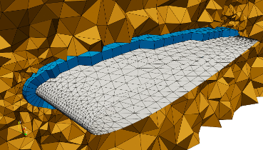
Fig 1. Linear Mesh with thick O-type prism layer(blue) and core tetrahedral mesh (yellow).

2. Input CAD

The second input is the CAD. This could be STEP/IGES/GEO file. One important feature of this NekMesh workflow is the capability to reconstruct the connectivity between the third-party mesh and the CAD. This brings a unique advantage that we can separate the linear volume mesh generation and its CAD from the CAD used in NekMesh for mesh curving and optimization. In this way, we can relax the requirements on the CAD quality in terms:

• No need to be Watertight (only a part of the CAD might be provided)
• Some CAD intersections are allowed
• Mesh Elements crossing two or more CAD Surfaces are allowed.

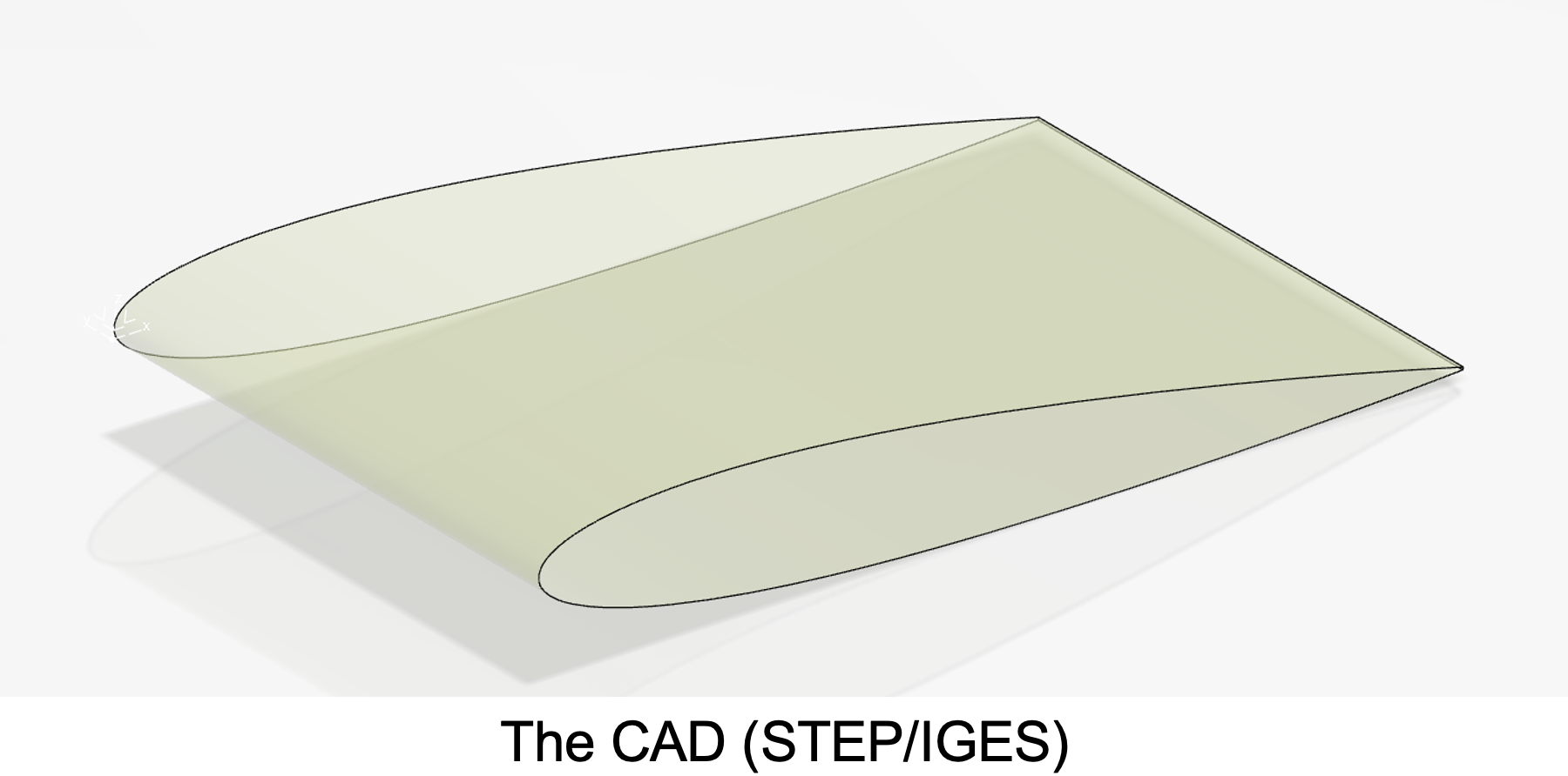
Fig 2. Example, where only the curved part of the CAD is provided.

Of course, the better the CAD definition, it is less likely there will be unexpected issues downstream the workflow.

To check the CAD you provide passes the minimum NekMesh requirements:

!NekMesh naca_linear.xml out.stdout -m loadcad:filename=NACA0012.stp -v -f

3. Mesh Curving and Surface Optimization

The core of the workflow is in the projectcad module. This will:

• Reconstruct the connectivity between the CAD and the mesh.
• Curve the mesh through projections of the mesh on the CAD
• Optimise the surface mesh

The method has a number of fail-safes ensuring that even bad CAD or poor linear meshes should be able to be curved. If the method encounters an issue, such as the linear mesh being a large distance from the CAD, it will simply leave that element straight sided. A well made CAD model and accurate linear mesh should be curved with little issue.

This module has been tested with:

• hybrid prism-tet-pyramid meshes
• fully hexahedral meshes
• fully tetrahedral meshes.

Let us now curve the NACA0012 mesh giving only the minimum necessary information - order of the polynomials that will be used to represent the curved geometry and the CAD file:

!NekMesh naca_linear.xml naca_HO.xml -m projectcad:file=NACA0012.stp:order=3 -v -f

Let us now try to analyse the log:

We first try to associate and project the vertices to their CAD. As we can see the Finite Volume mesher does not put them exactly on the CAD and hence $\delta_{max}$ $=1\times10^{-8}$ m .

• [ProcessProjectCAD] WARNING: Tolerances = 1e-06 1e-05
• ...
• [ProcessProjectCAD] - max surface Vertex correction 1.19209e-08
• [ProcessProjectCAD] - lockedNodes N= 0

This is way within our default tolerances and all vertices were succesfully associated (lockedNodes N=0).

In other cases, when working with very large geometries like full aircrafts, one might need to increase or decrease these, which will also speed up or slow down the association steps of the process. We provide a scaling cLength as a multiplier of these settings and an extension of the look-up around the CAD objects.

!NekMesh naca_linear.xml naca_HO-clength.xml -m projectcad:file=NACA0012.stp:order=3:cLength=100.0 -v -f

4. Volume Mesh Optimization and Mesh Untangling (Optional)

At this point we have already curved the mesh and have achieved a good geometrical accuracy for our p=3 coarse mesh. The mesh curving however can sometimes deform the elements, decrease the mesh quality and even cause some of them to self-intersect. Therefore, we could optionally apply our volume variational mesh optimizer varopti to improve the mesh quality and even untangle invalid elements.

The optimizer works by adjusting the positions of the all nodes to reduce a deformation energy. Intuitevely, by minimizing the deformation energy, the optimizer decreases the most distorted elements and produces a higher-quality mesh.

The flags that need to set:

• nq - (order + 1) from step 3
• maxiter - the maximum iterations you allow
• numthreads - multi-threading
• linearelastic - the type of energy functional

!NekMesh naca_HO.xml naca_HO_varopti.xml -m varopti:nq=4:linearelastic:numthreads=4:maxiter=10 -v -f

Note: This is the most memory heavy module of NekMesh. We recommend using high memory >64GB machine for large ($N_{el}$>1M ) meshes.

5. Ensuring Mesh Validity

In other cases, even after the application of the variational optimiser, you might still have several invalid(self-intersected) elements ($J_{sc}$ < 0.0). This could lead the simulation to diverge. There are many different ways to improve this like remeshing or refining this region, but this is out of the current scope.

Hence, you can just remove the high-order information (linearise) the few invalid elements and with that ensure the overal mesh validity:

!NekMesh naca_HO.xml naca_HO_valid.xml -m linearise:invalid -v -f 

As you already saw earlier, there are no invalid elements or highly distorted elements in our NACA0012 and no elements are linearised. However, with this module we can been certain the high-order mesh is valid and we can proceed with the final step.

6. Ensuring y+ resolution (Splitting O-type Quad/Hex/Prism Layer)

Remember that we created a single thick O-type prism layer around the body. At this point these prisms are curved and valid. So the final step is to ensure good resolution in also in the wall normal direction. We do that in the reference element with our bl module, which splits the macro prism, propagating the curvature inside the element. This guarantees that both the geometrical accuracy and mesh quality will be preserved.

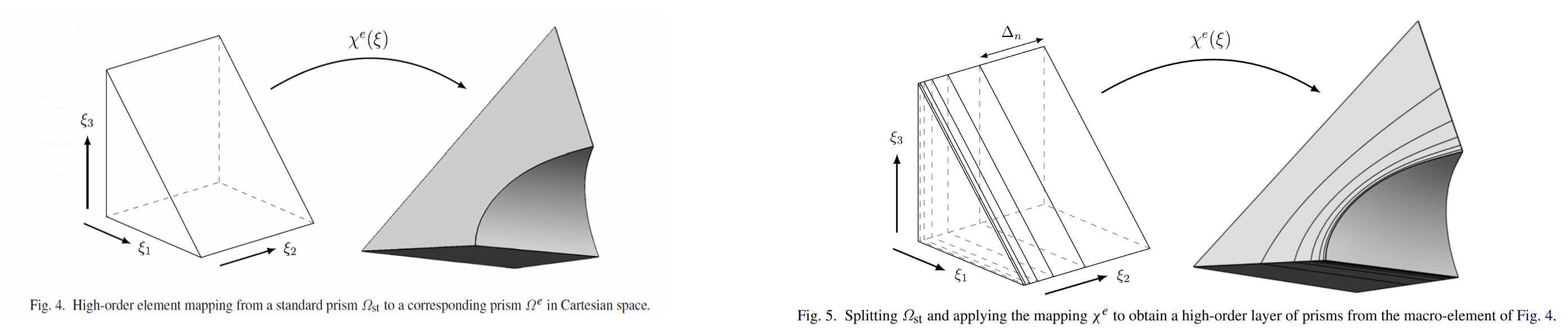
Fig 3. High-Order Splitting of Prism in the reference element, propagating the curvature inside.

The arguments that bl requires are:

• nq - (order + 1) from step 3
• layers - number of boundary layers
• r - relative progression ratio between layers
• surf - mesh composites to be split

Here to understand what surfaces(composites) we would like to target, we open one of our XML mesh files and progress to the end of the file:

<COMPOSITE>
    ...
    <C ID="7" NAME="Wing">
    ...
</COMPOSITE>

In this case we are lucky as the composite surfaces have names and we know we would like to resolve the flow around the wing, hence surf=7. When not refer to step 8.

!NekMesh naca_HO_valid.xml naca_HO_valid_bl.xml -m bl:nq=4:surf=7:layers=5:r=1.5 -v -f

7. Visualize Mesh with Paraview

To visualize the high-order mesh, we can use our post-processing utility FieldConvert.

!FieldConvert naca_linear.xml naca_linear.vtu -n 2 -v -f 

!FieldConvert naca_HO.xml naca_HO.vtu -v -f 

!FieldConvert naca_HO_valid_bl.xml naca_HO_valid_bl.vtu -v -f 

Additionally, we can visualize the element mesh quality ($J_{sc}$) by using the qualitymetymetric FieldConvert filter and a Threshold criteria in Paraview to extract only the deformed ones. This could help with their mitigation for complex geometries.

!FieldConvert -m qualitymetric:scaled naca_HO.xml naca_HO.vtu -v -f 

We can now open the meshes in Paraview. (slow on the Virtual Machine)

!paraview naca_linear.vtu naca_HO.vtu naca_HO.vtu -v -f 

Some important points to note in the visualisation of high-order meshes and fields:

• This visualisation shows a linear representation of the mesh. That is, inside each element, we are sampling the coordinates at discrete points and then performing linear interpolation between these. Therefore lower-order simulations may look jagged when the underlying error is actually rather small.
• Owing to this, in the visualisation above, you are viewing all integration points of the element. In triangular elements in particular, this can be somewhat visually odd: in Nektar++, we utilise a collapsed coordinate system to represent triangles, where two corners of a quadrilateral are merged into one. Thus the distribution of points within a triangular element is 'squashed' in one direction.

8. Extract and Visualize Surface Mesh

Sometimes during the post-processing, validating of the meshing or just to identify the correct composite ID, we would like to extract the high-order surface mesh. We use the extract module, with the surf being the Composite IDs of the mesh, as in Step 6 for example.

!NekMesh naca_HO_valid_bl.xml naca_HO_valid_bl_surf.xml -m extract:surf=7,8 -v -f 

This becomes a 2D manifold mesh. Then we can convert it to vtu with FieldConvert and visualize Paraview.

!FieldConvert naca_HO_valid_bl_surf.xml naca_HO_valid_bl_surf.vtu -n 10 -v -f 

To visualize the real NekMesh geometrical accuracy, we have also uploaded a mesh with high-order VTK visualization. You can open it on your personal PC with Paraview installed and in general convert with FieldConvert with the flag vtu:vtu:highorder. This requires to build Nektar++ from source with NEKTAR_USE_VTK ON.

!paraview naca_HO_valid_bl_surf_complete.vtu

9. Export Meshes to external solvers

Nektar++ formats:

• .xml (Nektar++) - main internal format
• .nekg (Nektar++ HDF5) - large scale Nektar++ simulations

External formats:

• .msh (GMSH format) - recommended
• .vtk (linear mesh only)
• .stl (linear surface)
• .stdout (no output file)

!NekMesh naca_HO_valid_bl.xml naca_HO_valid_bl.msh -v -f 

In case, your solver requires different polynomial order for the solver than the one used during curving, you can export the mesh with a uniform polynomial order. This applies for all high-order output modules and does NOT improve the geometrical accuracy. This is not necessary if you use Nektar++.

!NekMesh naca_HO_valid_bl.xml naca_HO_valid_bl.msh:msh:order=4 -v -f 

Take-a-ways:

It is worthy to keep in mind the following points:

• NekMesh can generate high-order curved meshes with our state-of-the-art high-order modules from third-party external meshes.

• This workflow is applicable also for very complex geometries.

• No watertight or perfect CAD is necessary for this workflow.

• Currently, we recommend creating thick O-type prism layer meshes around the body and core tet mesh. (Some new functionalities incoming.)

• Visualization of curved meshes can be performed with Paraview

• If in the future you build from source add the following additional flags in ccmake when building Nektar++:

  • NEKTAR_USE_MESHGEN ON
  • THIRDPARTY_BUILD_OCE ON (or build it yourself)
  • NEKTAR_USE_VTK ON (Optional for vtu:vtu:highorder visualization)
  • NEKTAR_USE_CCM ON
  • NEKTAR_USE_CGNS ON